
Global equity markets have been under huge pressure in recent months. The closest technical pattern could be observed in the beginning of 2000, when the dot-com crash happened. We have highlighted this phenomenon several times. By now the equity market turned out to be even more negative than it was twenty years before. It is almost presumed that the recession is coming, so stocks start pricing in the worst scenario. In our opinion the recession is possible indeed, but investors tend to be more downside looking than the situation implies. We decided to dig deeper in technical and fundamental features of the dot-com crash and current market.
Introduction
Figure 1 compares NASDAQ index in 1996—2003 and the present behavior of ARK Innovation ETF (the ‘ARK’) consisting mostly of technology and biotech stocks. Apart from the visual similarity of the two charts there are several other common features:
1. Both NASDAQ and ARK represent the ‘hottest’ market segments
2. NASDAQ rally started in 1999 – after a long-lasted bull market that had begun in early eighties. Investors got focused on the riskiest market segment after all other stock had become overpriced. We can see the same pattern with ARK
3. Both rallies happened right after the economy crises: the Asian and Russia crisis in 1998 and the COVID-19 crisis in 2020. It looks like the market corrections in both cases triggered investors to pay attention to the fast-growing companies.
Figure 1
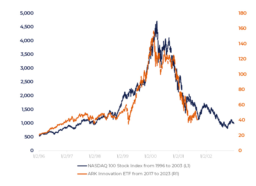
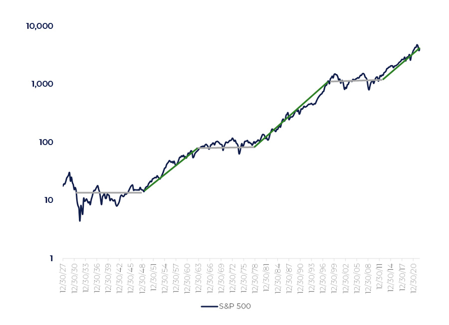
Figure 2 demonstrates the cyclical nature of US stock market: we can visualize it as a sequence of stagnation and growth cycles. The average lifespan of bull markets is 15—20 years. By now we have been living in an uptrend for 10—12 years depending on which starting point we take. So, we are coming close to the finish point of the growth period with patterns of 2000 and 2022 being quite similar.
On top of that, the US Federal Reserve (the ‘Fed’) is conducting the monetary tightening policy. In his speech in Jackson Hole, chief of Fed Mr. Powell said, “there will still be a pain to households and businesses”. The inflation has climbed to its 40-years high, hence, regaining price stability requires radical steps from the Federal Reserve. To be precise, there is only one step – lifting the base rate to a restrictive level at which taking new loans becomes too expensive.
Investors are worried that lifting the base rate too high might lead to a recession.
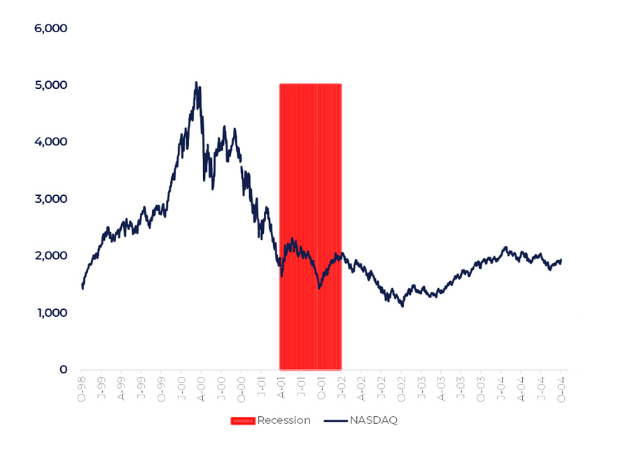
According to the Figure 1, ARK is now in relatively the same place as NASDAQ was in September 2001. The US economy was in recession between March 2001 and January 2002. The equity market, meanwhile, reached its local bottom closer to the end of the recession, in September 2001 (Figure 3).
Figure 2
It is frightening that the equity and bond markets have corrected substantially with the recession not having started yet. Moreover, so far there are no signs it will start soon. In the post-World War II period, from 1945 to 2020, the average recession lasted about 10 months. This creates quite cloudy investment environment. At first, stocks can be under pressure because of the recession expectations and then because of the recession itself. Moreover, the pattern of 2001 demonstrates that even after the economy returned to normality stocks were remaining under pressure during the whole 2002 (Figure 3). That extends the downtrend’s lifetime even more.
Figure 3
There is another perspective of the same picture, though. Perhaps, the stock market has already priced in the recession scenario and the further downside is limited. The Figure 1 shows that the US equity market is so low as if the recession is underway. Stocks’ behavior will depend on how likely the upcoming recession is and how deep it can be.
Inflation pressure
What is happening now is that people are paying for the support measures provided by the US Government during the pandemic period. Those measures are nothing but monetary emission. The M2 as of mid-2022 is 40% higher than it was before the COVID-19 outbreak.
According to the famous equation this means that prices should go up 40% also :
(real GDP)*(price level in economy)=M2*(money velocity)
[1] Money in circulation [1] More strictly, this is correct if the money velocity and the GDP are constant
Figure 4
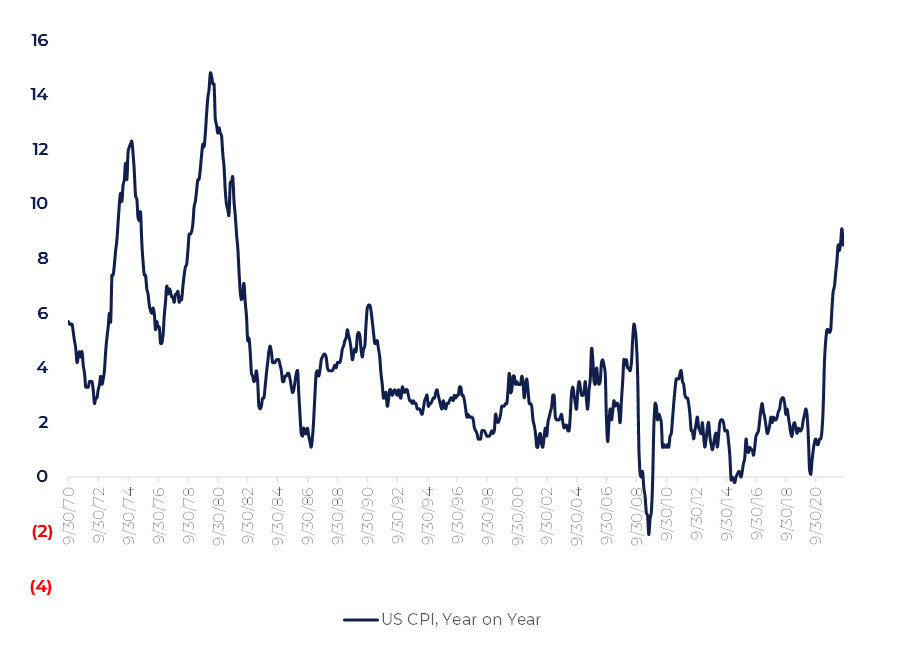
Indeed, prices have grown up significantly already. US inflation has reached 9% (Figure 4), which is a record level for the past 40 years.
It is widely known that high inflation motivates businesses and households to take loans if the loan rate is lower than the inflation. This leads to rapid M2 expansion and, eventually, to hyperinflation. To contain credit expansion Central Banks rise key rates. According to the general practice , the key rate should be larger than the inflation. Since March 2022 US Consumer Price Index (CPI) has never been below 8%. Such a level of the key rate seems unbearable for the economy.
Even without possible monetary expansion there is already extra 40% of printed money. This surplus should dissolve in the economy pushing prices up.
How to measure inflation?
The two most popular concepts are:
– CPI (Consumer Price Index)
– PPI (Producer Price Index)
[3] One of the mostly known principles of targeting inflation is referred to as “Taylor Rule”.
CPI concept is based on an average market basket of consumer goods and services purchased by households. PPI measures the average changes in prices received by domestic producers for their output. Both figures are calculated by the Bureau of Labor Statistics .
Figure 5
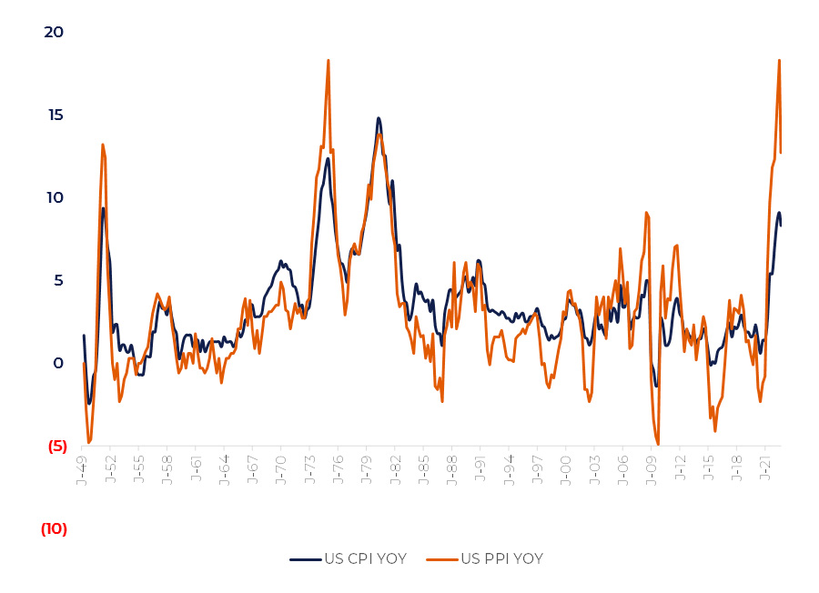
PPI is more volatile than CPI (Figure 5). More precisely, it is about three times more volatile. A revenue of a typical company producing consumer goods is sensitive to CPI while costs are sensitive to PPI. Figure 6 compares ⅓ of US PPI to CPI – the difference is very small. It shows how swings in consumer prices influence expense prices and vice versa.
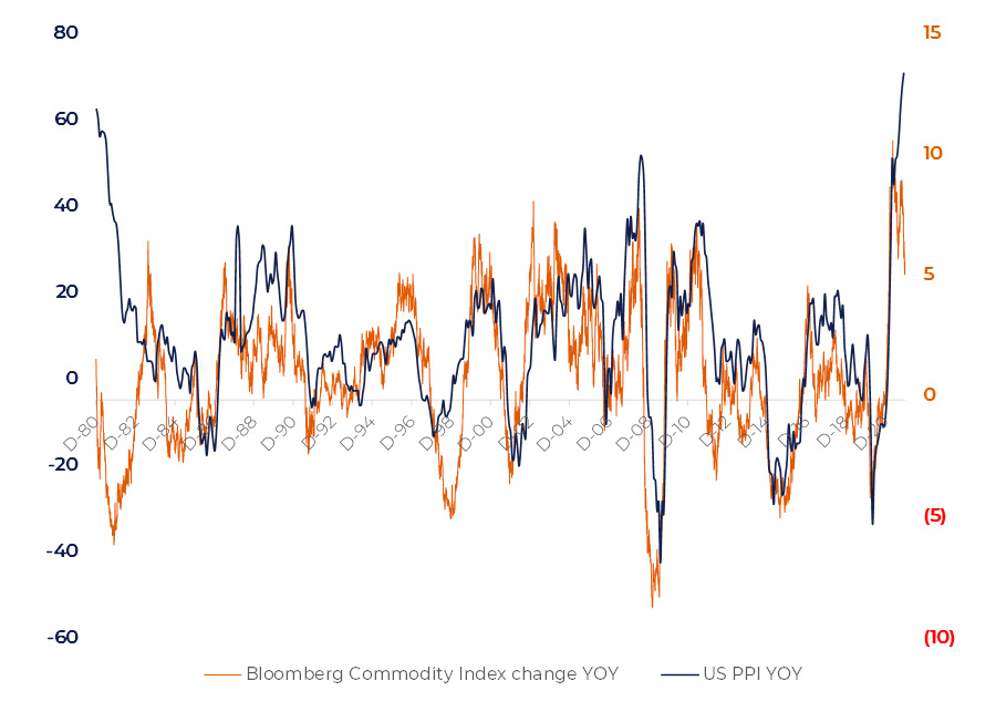
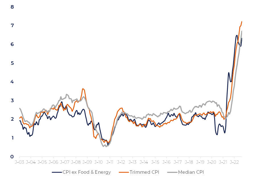
Another important feature of PPI is its strong correlation to commodity market (Figure 7). Commodities also impact CPI through CPI—PPI relation. Calculating inflation without volatile Food and Energy components is referred to as “core CPI”. Besides ignoring Food and Energy the Fed also uses concepts of “Trimmed CPI” and “Median CPI”. All these methods use different approaches to eliminating volatile components.
[5] The description is available on a Fed Bank of Cleveland webpage: https://www.clevelandfed.org/our-research/indicators-and-data/median-cpi.aspx
Figure 6
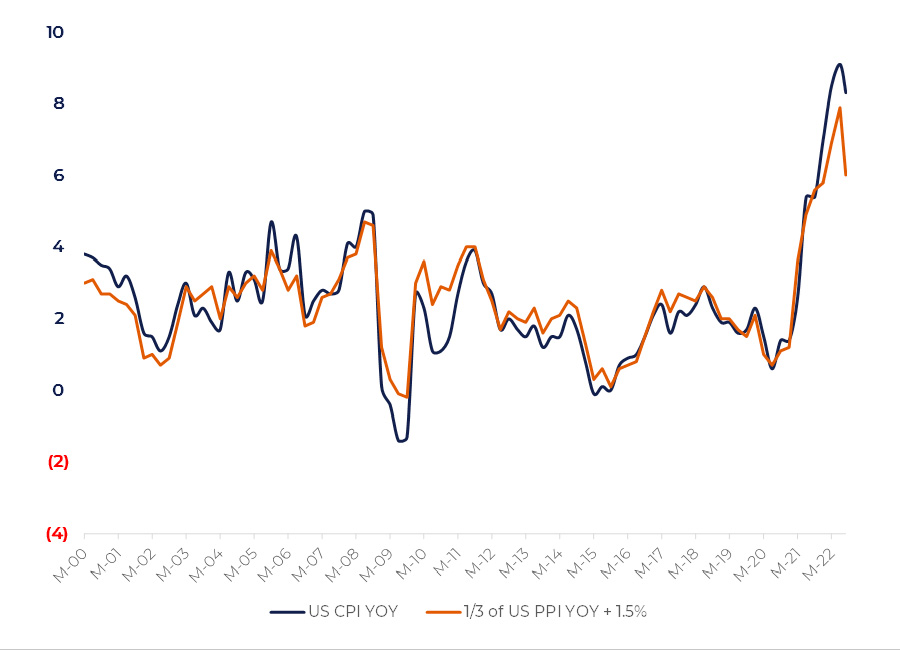
Figure 7
The difference between all these methods is not principal, so we will use the term “core inflation” with respect to any smoothing algorithm.
Figure 8. Core inflation aggregates
Besides CPI, which is calculated by the Bureau of Labor Statistics, there is another widely know consumer inflation measure: PCE: Personal Consumption Expenditure index calculated by the Bureau of Economic Analysis. Since 2012 the Fed has taken PCE as a major inflation gauge.
There are two major differences between these two inflation figures:
– PCE consumer basket is reconsidered every month unlike once every two years in case of CPI
– PCE accounts for indirect consumer spending such as employer’s medical insurance, various government services etc.
– CPI generally tends to be higher than PCE since consumers change their demand structure as prices grow. They decrease consumption of expensive goods and services in favor of cheaper ones (Figure 9).
Figure 9
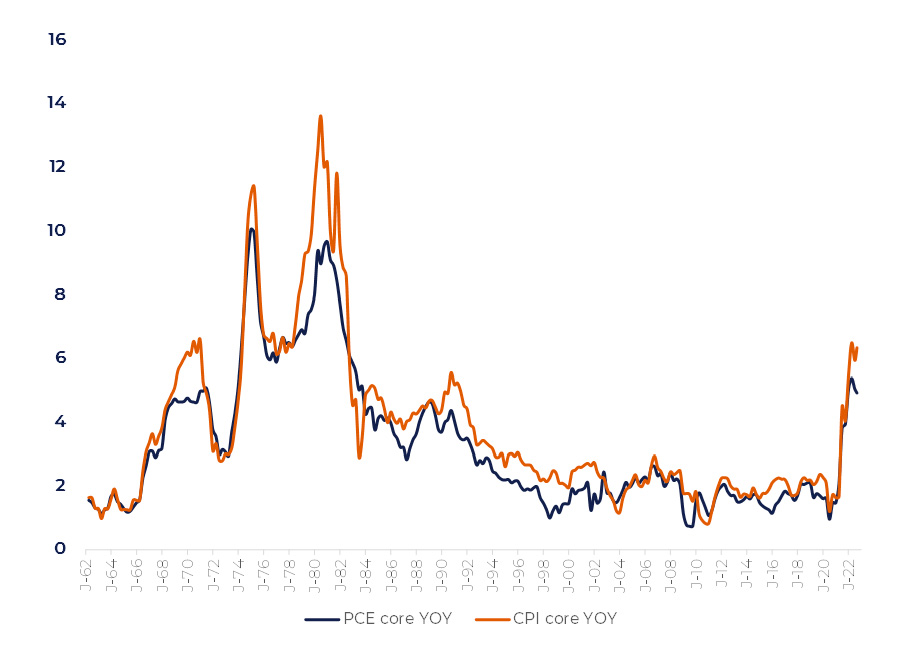
Figure 10
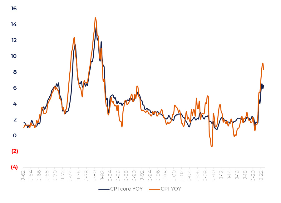
Core inflation is generally slow-moving, it behaves like a moving average of total inflation (Figure 10). When the course of inflation reverses the total figure is almost always a leading indicator for a core gauge: it generally takes one or two quarters for the core inflation to follow the total figure. The Fed prefers using slow-moving core indicators to achieve predictability of its policy.
For trading purposes, gross inflation is important because of its predictive ability.
Both CPI and PPI seem to take the course downwards. As it was shown PPI is a derivative of commodities behavior with CPI strongly correlating to PPI. Fundamentally PPI is going to decrease as in Q1 2023 PPI will be affected by the high base effect on the commodity market. Before that the inflation gauges will fluctuate with consequent positive and negative surprises. This will probably force the Fed act more aggressively to suppress the price rise.
For further investigation we will break the inflation pressure into three components:
– Monetary pressure. It emerges once an excess of money has been injected into economy.
– Consumer confidence. It tells us how confident consumers are to spend their savings.
– Inflation expectations. It tells us to what extend households and businesses suppose the price rise is rational.
Monetary pressure
Figure 11 shows the ratio of M2 to the nominal GDP:
Figure 11
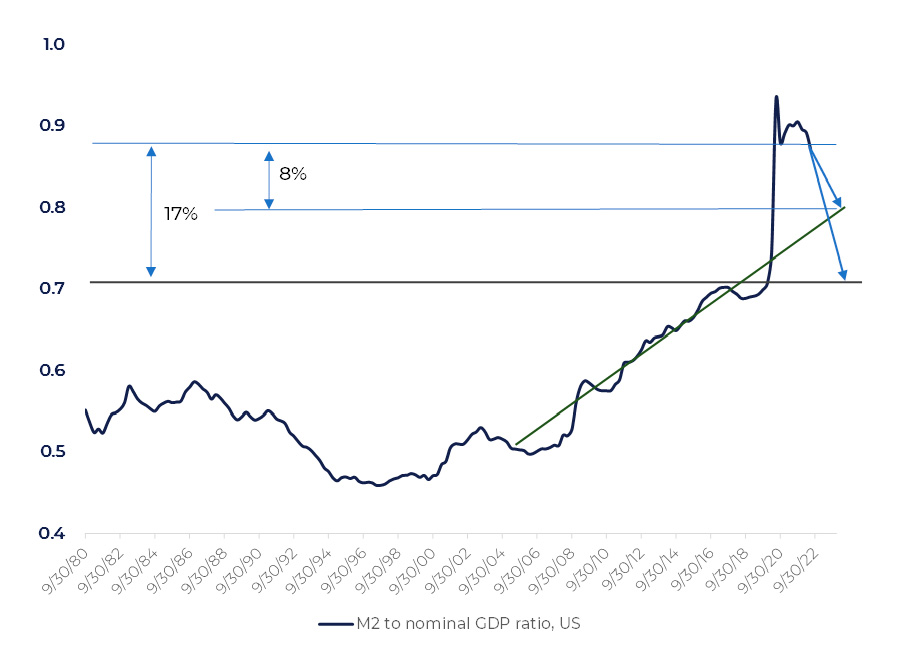
Support measures drove M2 well above the pre-COVID levels. Inflation led to the nominal GDP growth of 15%, partly offsetting the monetary surplus in the economy. By the end of 1H 2022 the monetary excess had stabilized at 17% level above the pre-pandemic level.
We should keep in mind that M2/GDP ratio has been growing since 2000, as Figure 11 demonstrates. If this trend persists the economy will need to digest 8% of M2 by the end of 2023. In other words, after the price growth of 8% the economy will come close to balance in monetary terms.
Now let us assume that the Fed will succeed with its fight, and we have CPI of 2% at the end of 2023. In the simplest interpolation CPI will go down from 9% in Q2 2022 to 2% in Q4 2023, resulting in the average inflation of 5.5% over this period. In absolute terms prices will go up by 5.5*(1.5 years) = 8.25%.
This logic works when the real GDP and M2 are both constant. GDP growth helps to absorb extra money while M2 expansion works in the opposite direction. Gradual decrease of CPI to 2% by the end of 2023 with these assumption looks realistic. The weak point of such approach is that the uptrend of M2/GDP ratio is just an assumption, not the fact.
The worst-case scenario is that the economy should absorb the whole amount of 17% excess of money (Figure 11). In this case even after bringing inflation down to 2% there still will be another 8—9% of monetary excess.
Figure 12
Whether or not the absorption of 8% of monetary mass is sufficient we will only see closer to 2024. Until then the most important factor will be the Fed’s ability to put the core inflation under control.
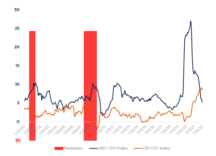
In case the Fed overplays with tightening and causes a recession, the inflation issue will cease to exist. The cases of 2001 and 2008 recessions demonstrate that CPI dropped within those periods even being accompanied by 15% M2 expansion (Figure 11).
In case of soft-landing the monetary pressure will get weaker with the time: the nominal GDP will be growing in line with inflation so that at some point it will strike a balance with money in circulation.
Consumer confidence
Figure 13 displays the consumer sentiment indicator measured by the University of Michigan.
Figure 13
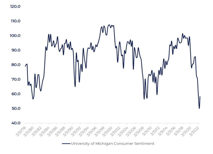
It is quite a paradoxical fact that the consumer sentiment is so low while the unemployment (Figure 20) is at its record low too. It is noteworthy that the low sentiment is often accompanied by high inflation mirroring difficulties consumers face in planning their spendings.
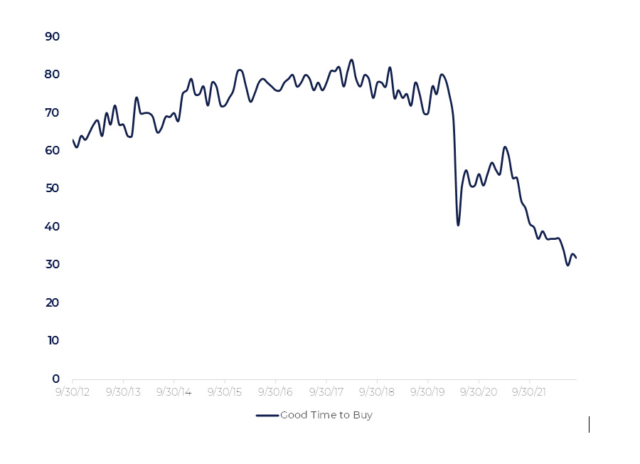
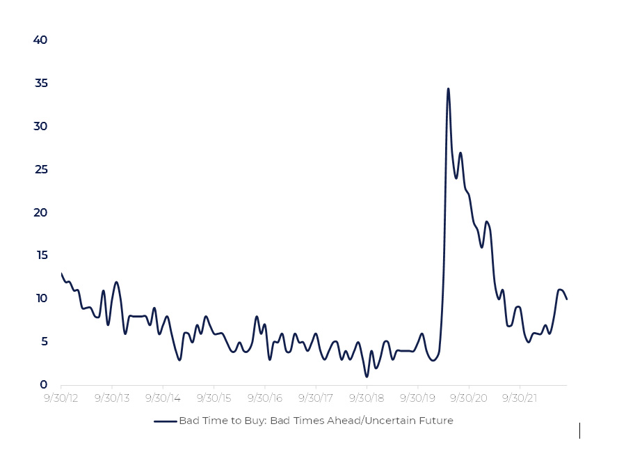
University of Michigan Consumer Confidence review shows that in August 2022, only 30% of respondents considered their current financial situation as “better off” vs 1 year ago. Before COVID, this metric was above 50%. Figure 14 reflects how households evaluate buying conditions for large household durables. However, the share of individuals thinking about “bad times ahead” is comparatively small (Figure 15). That means that individuals are ready to spend money but cannot afford to buy durables because of high prices.
Employment stability seems to be the main driver of extra spendings. J. Powell pointed out in his speech at Jackson Hole that the Fed’s actions will “soften” the labor market. It is unlikely, though, that individuals will reduce their spendings just based on Mr. Powell’s speech. While unemployment is close to its historical bottom, one cannot expect a visible change in demand from individuals.
Figure 14
Cooling down the labor market is hard without hitting businesses. Companies are much more reluctant to invest in growth (See chapter “Common features and differences between 2001 and 2022 patterns”). However, they are actively hiring people pushing wages up. It looks like firms are aware of upcoming hard times but have much cash. Extra Capital Expenditures is dangerous, but hiring is much less riskier because extra staff may always be laid off.
Figure 15
Banks have already taken into consideration the key rate expectations, so the actual loan rates are already high enough. US mortgage rates have exceeded 6%. By now this has only marginally reduced the demand pressure on prices. The main factor supporting consumer demand is solid labor market. Individuals might take loans to buy expensive goods as they are confident in their ability to find a new job, perhaps with higher salary (see chapter “Labor market”).
The history of a “Bad Times Ahead” indicator shows it reaches peak levels during recessions. That was the case in 1980, 1982, 1990, 2001, 2008 and 2020. It strongly correlates with unemployment which always comes in parallel with recessions also (Figure 35). The historic evidence shows that unemployment cannot be managed in manual mode. It is either uncontrollably soaring or stable.
To sum up, we cannot expect that the Fed’s actions will affect consumer confidence unless hard landing happens and unemployment surges.
Inflation expectations
Inflation expectations are always based on past experience.
It allows economy to operate properly right after the money excess emerges.
Figure 16
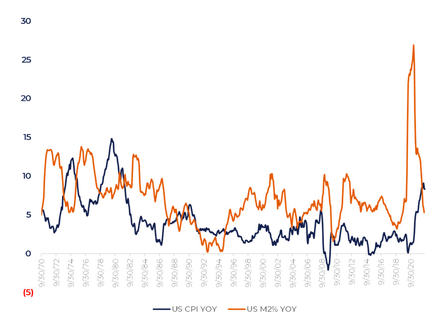
Figure 16 demonstrates that US CPI turned down 2—3 years after M2 expansion had reached its peak in 1970s. Now the inflationary processes are moving faster. As inflation began to rise in March 2021, the Fed’s Chair Powell predicted that the increase would be “neither particularly large nor persistent.”
Powell’s view was supported by the many economists on Krugman’s (2021) “Team Transitory” . It is now understood that the inflation is much higher than the Fed expected. Apart from the supply chain disruptions, fast exit from the COVID restrictions, and high commodity prices sparked by the Russian-Ukraine war, the Fed points to a dramatic increase in the job vacancies-to-unemployed ratio, which was unexpected and did not occur until late 2021.
[7] https://www.bloomberg.com/news/articles/2021-03-23/powell-expects-inflation-to-bump-up-but-it-won-t-get-out-of-hand#xj4y7vzkg
[8] https://bcf.princeton.edu/wp-content/uploads/2022/01/Webinar-Transcript-2.pdf
We may break the recent history of US economy starting the outbreak of COVID into two periods:
1. Massive monetary stimulus (40% of M2 expansion) but low inflation expectations: partly due to the past experience, partly because of the pandemic-related uncertainty in the economy.
2. Reduction of the money excess from 40% to below 20% causing the reduction of monetary pressure coming in with high inflation expectations formed by soaring prices.
The danger of high inflation expectations is that they may become entrenched influencing the way households and businesses take decisions. It creates upward prices pressure, opposite to the downward pressure causing by the reducing monetary excess in the economy. Bringing down inflation expectations is the major objective for the Fed today.
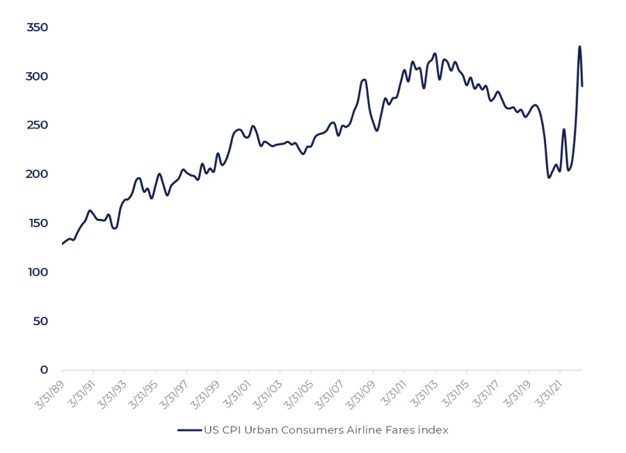
The consumers’ demand is limited by the amount of money in the economy. If monetary supply is not growing prices will not go too high, otherwise the gap between supply and demand emerges. This gap drives prices down until a balance is found. US CPI Airline Fares is a typical example of this pattern (Figure 17):
Figure 17
The Fed regulates the amount of money in the economy through setting a key rate. Eventually, M2 is a product of banks’ lending. To contain M2 expansion the key rate should be restrictive enough to prevent credit expansion.
Figure 18
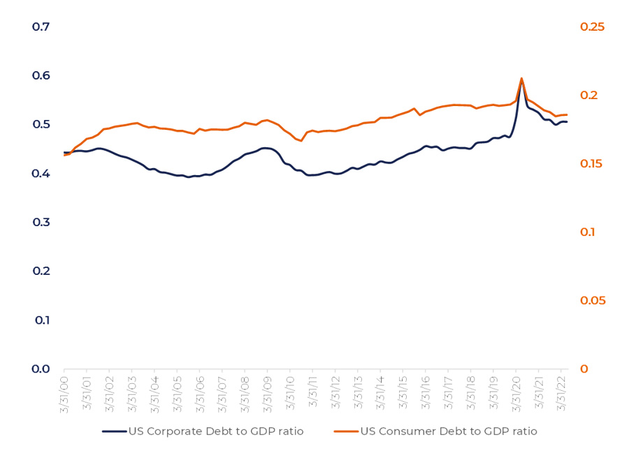
Both US corporate and household debt have been declining compared to GDP over the past 2 years (Figure 18). In 2022 both ratios stabilized.
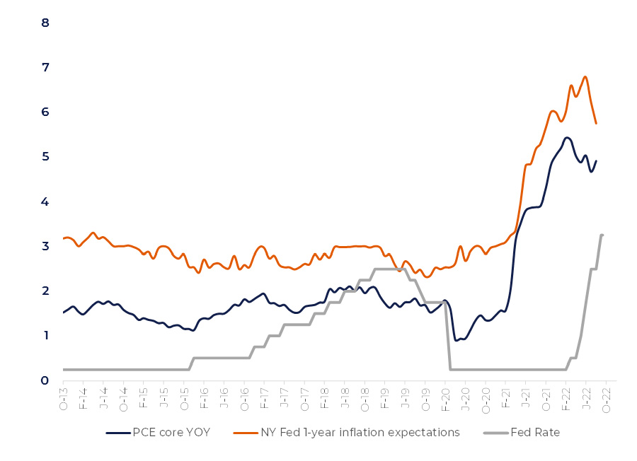
M2 has stabilized as well (Figure 16 demonstrates the slowdown of M2 expansion). However, the key rate is still lower than the inflation and, which is more important, than inflation expectations (Figure 19) . Even if the gross CPI has reversed, the slow-moving core inflation will remain at a high level until the beginning 2023. However, the spread between the key rate and inflation expectations is narrowing. In case the expectations will dive under the key rate, the situation will become much more certain.
[9] There are various inflation expectations calculation methods. In this case 1-year consumer NY Fed survey inflation expectations is taken for considerations. Longer term expectations are significantly lower.
Figure 19
Before 2023 the Fed’s public statements are probably more important than the key rate itself. Since the Jackson Hole conference the Fed’s rhetoric has become extremely hawkish. Besides the key rate level guidance, the Fed emphasizes that the restrictive policy will last long. Banks, knowing that the key rate will be higher for long, raise their lending rates in advance, considering several upcoming rate hikes. For 2022 two-years US Government bonds’ yields have been sustainably higher than the key rate by 1—2%.
As Fed’s Chair Powell stated in his speech in Jackson Hole “Our responsibility to deliver price stability is unconditional”. Investors read between lines that the Fed will keep high rates even if it causes a recession. This also discourages firms from borrowing.
Such approach helps the Fed form inflation expectations. If hawkish rhetoric is used by the Fed as a partial substitute for the rate hike, it will prevail until at least Q1 2023 when the direction of the core inflation will be clearer and more certain. It is worth noting that the more depressed picture the Fed manages to paint, the less damage to the economy from the rate hike will be made.
Fed’s view on the situation
Strangely enough, the Fed is trying to avoid mentioning the relation between COVID monetary stimulus and the inflation issue. Instead of that the Fed is pointing to the hot labor market and imbalance between supply and demand in the economy.
Labor market
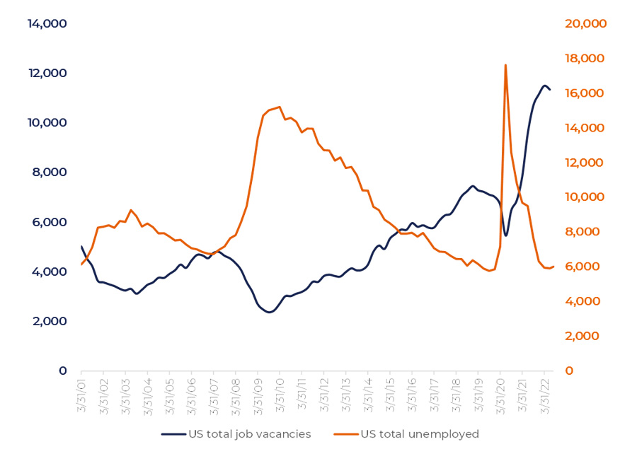
The US unemployment rate has reached its record lowest level after the COVID restrictions were largely released. The number of open vacancies in US labor market has surged disproportionally more (Figure 20):
Figure 20
The way the Fed considers the influence of the labor market on inflation is described in an article written for the BPEA Conference held in September 2022 .
[10] The Brookings Papers on Economic Activity (BPEA) is a semi-annual academic conference and journal that pairs rigorous research with real-time policy analysis to address the most urgent economic challenges of the day. The mentioned article can be reached through the link: https://www.brookings.edu/wp-content/uploads/2022/09/Ball-et-al-Conference-Draft-BPEA-FA22.pdf
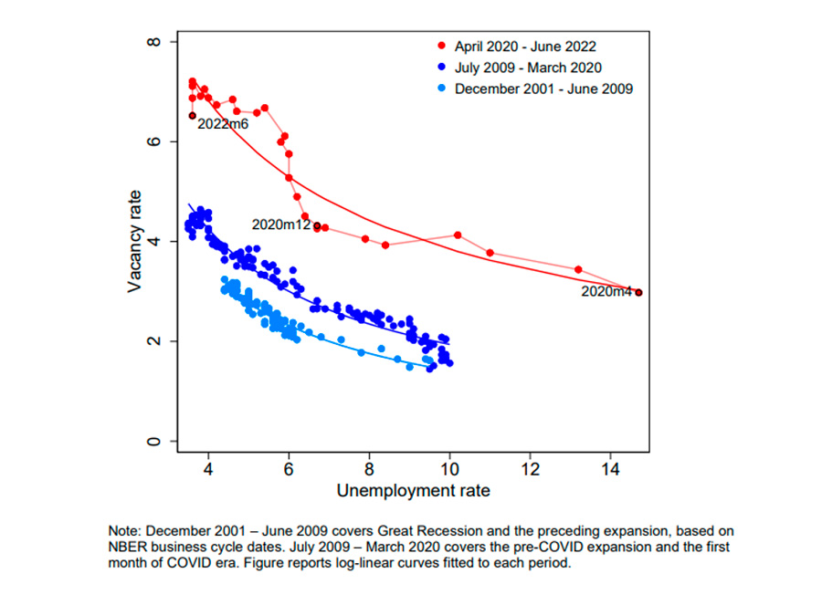
The unemployment depends on the number of open vacancies. This dependence is known as Beveridge curve and shown on Figure 21:
Figure 21
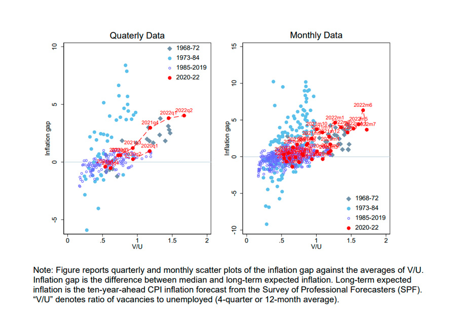
For further calculations the authors take Median (or core) CPI cleaned off volatile components and compare it to the inflation expectations (Figure 22). The difference between the core inflation and inflation expectations is referred to as inflation gap. Inflation gap is a function of:
– Headline (or CPI) inflation shocks (inflation volatility)
– (V/U) ratio which is labor market vacancies divided by unemployment
Figure 23 reports quarterly and monthly scatter plots of the inflation gap against the averages of V/U.
[11] Figure reports 10-year-ahead CPI inflation forecasts from the Survey of Professional Forecasters (SPF)
Figure 22
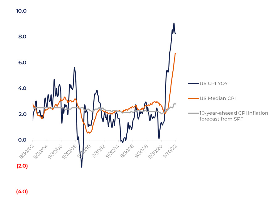
Figure 23
Knowing the way CPI gap depends on V/U ratio and the form of the Beveridge curve (Figure 21) one can calculate the way CPI gap depends on the unemployment rate (Figure 24) :
Figure 24
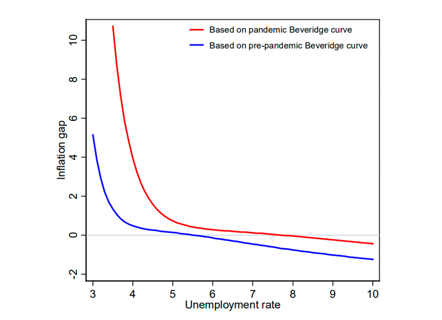
The first thing to be mentioned is that pandemic and pre-pandemic Beveridge curves are different reflecting the mismatch between professional skills of unemployed people and the structure of demand on labor force from the side of employers.
The second observation is that the inflation gap only reduces when the unemployment rate goes up above 4%.
Further assumptions are that the unemployment goes to 4+% area with CPI moving towards 2% area target without new inflation shocks. These assumptions allow to compute the future inflation gap (Figure 25) in optimistic and pessimistic scenarios.
The difference between optimistic and pessimistic scenarios depends on what Beveridge curve is taken. If a mismatch between the employers and unemployed persists much higher inflation will come out. If a Beveridge curve reverts to its pre-pandemic form the labor market will cool down and help the Fed keep the situation under control.
[12] this logic (aka Philips curve) did not work during 70s stagflation in the US. See: https://www.federalreservehistory.org/essays/great-inflation
Figure 25. Scenarios for Core CPI Inflation Conditional on June 2022 FOMC Unemployment
Forecasts (12-month; percent)
Those wanting to go deeper into the Fed’s logic may follow the link in the Footnote 10.
For our purposes we would like to highlight a couple of details:
– The Fed focuses on the core inflation which is a lagging and slow-moving indicator. Markets correlate to the gross CPI which includes volatile components. The core figure does not have predicting power.
– Fed ignores monetary factors as if the labor market is nearly isolated from them.
It is obvious, though, that the high vacancy rate is a consequence of the monetary excess in the economy. Figure 26 reveals their correlation. If the money access ratio cools off as it is demonstrated on Figure 11 the labor market would come close to its neutral level as well.
Figure 26. Vacancies-to-unemployed ratio vs Money excess
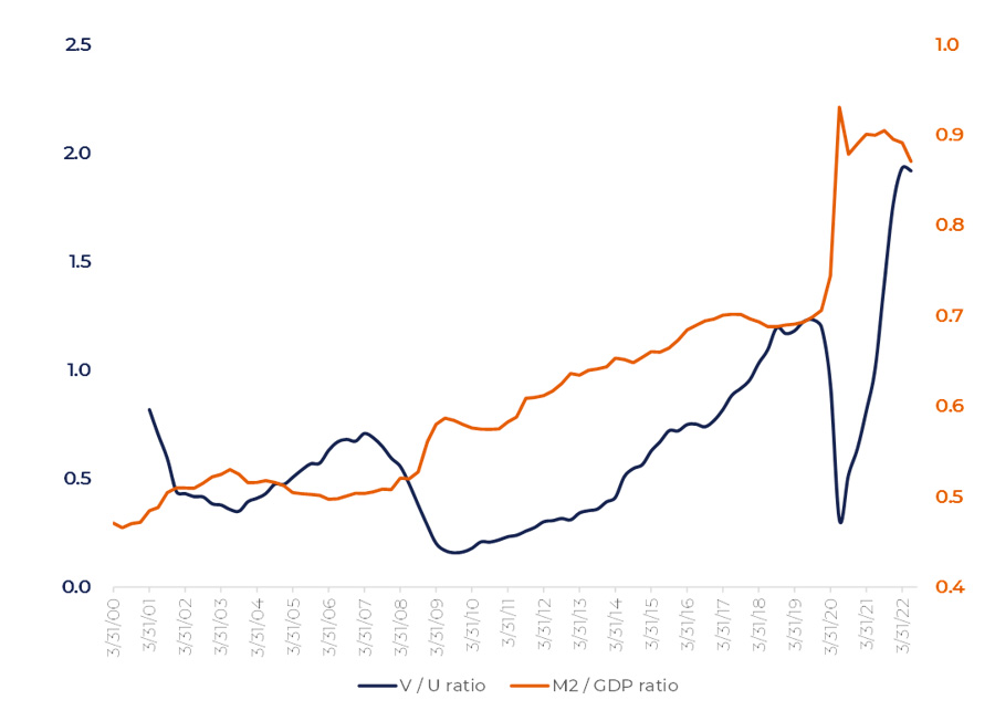
Figure 27
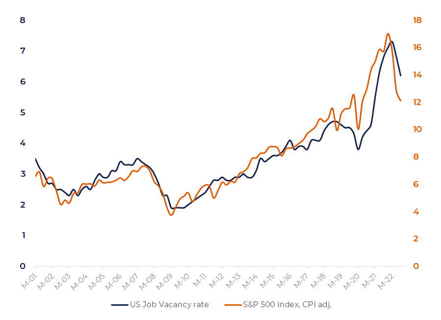
Interestingly, the equity market behavior and the US Job Vacancy rate looks strikingly similar (Figure 27). This comparison shows that the equity market has overreacted, pricing in almost full potential drop in vacancies.
In our view, investors underestimate the role of vacancies in fighting inflation. It is the vacancy rate that has driven V/U ratio out of balance. Returning to equilibrium will also be achieved through the job vacancies contraction. We do not know what unemployment rate we will get in the equilibrium point. The simplest assumption is that the unemployment rate will reach its pre-pandemic level which is exactly what we have now.
Most probably the unemployment will grow to 4+% area due to the damage caused by high interest rates. Fed’s point of view is based on the statistical data from the 1985—2020 where the unemployment ratio under 4% was outlying.
A separate question is whether the uptrend in the vacancy rate is sustainable (Figure 20). Growing vacancies can be a consequence of structural changes of US economy which is going more global and requiring employees with contemporary skills. On the other hand, from a historical perspective, the unemployment rate below 4% is a rare phenomenon. Over the past 70 years it only was in that area four times: in 1951—1953, 1965—1969, 2018—2019 and now. We have too small statistical data to be sure that the 4-% unemployment ratio always comes along with the overheated economy. Equally, we cannot state otherwise.
Supply-Demand balance
The nature of current high-inflation environment can be considered as a state of economy when employed people are seeking to buy more goods and services than they can produce.
Fed Chairman Powell has highlighted it many times that the Federal Reserve only deals with demand, not supply . It is noteworthy, though, that supply chains constraints coupled with the energy crisis are the major factors resulting in soaring inflation. Despite being at historically high levels, global supply chain pressures have been decreasing since January 2022.
[13] “It is also true, in my view, that the current high inflation in the United States is the product of strong demand and constrained supply, and that the Fed’s tools work principally on aggregate demand. None of this diminishes the Federal Reserve’s responsibility to carry out our assigned task of achieving price stability. There is clearly a job to do in moderating demand to better align with supply. We are committed to doing that job.” — J. Powell speech at Jackson hole, 2022, Aug 26. https://www.federalreserve.gov/newsevents/speech/powell20220826a.htm
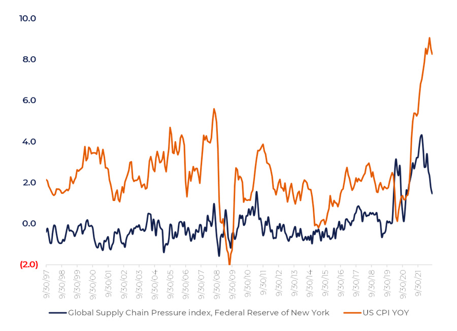
Figure 28 demonstrates correlation between global supply chain health and US inflation.
Baltic Dry index rocketed to 5000 in September 2021 from its average sustainable level at around 1000 over 2010—2020. By September 2022 it has gone down back to 1’500 area. In reporting calls for Q2 2022 we can find that many companies stated that the supply chain disruptions remained in the past.
In summer 2022, the airline fares soared on fast demand recovery with the airline companies being understaffed by 10% on average . Despite the crunch in airline services companies are not in a hurry to hire new staff at any cost.
Figure 28
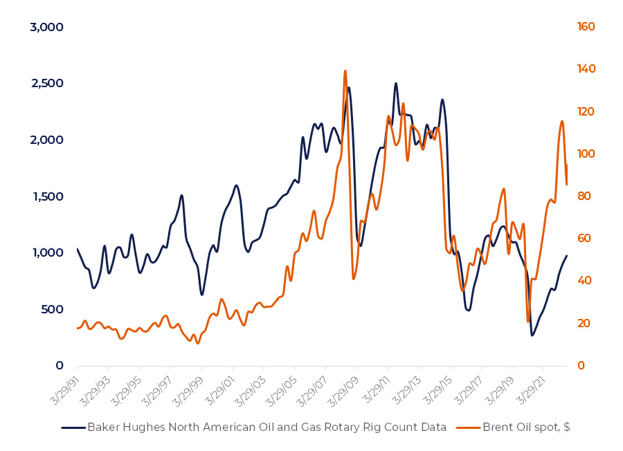
We can notice the same trend in the Energy sector where companies do not enhance spendings on infrastructure despite an enormously high level of oil and gas prices. New shale oil and gas drilling is still lower than in 2017—2019 period (Figure 29).
[14] It demonstrates, by the way, the nature of the Beveridge curve upward shift. The record low unemployment tells that former airline workers managed to find jobs in other sectors. COVID led to a surge in vacancies related to the online trading and delivery.
Figure 29
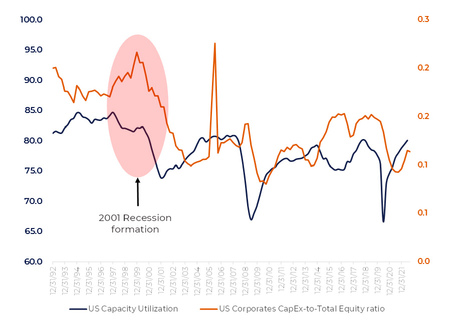
This reflects corporates’ pessimistic view on developments in global economy in the forthcoming years. The monetary excess, being a negative factor from an inflationary perspective, is supporting solid demand. On the back of low fixed investments, the capacity utilization in the US economy has returned to its pre-pandemic top level of 80% (Figure 30). The industrial production looks very good as well.
Figure 30
The issue is that, though, the economy cannot produce enough goods and services even working at full capacity. In a balanced economy the labor force produces as much as it consumes. Now there is a share of working force with close to zero contribution to GDP.
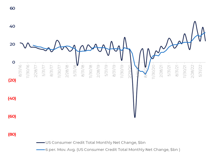
Being confident about their future and seeing solid labor market consumers maintain their borrowing activity at a high level (Figure 31). The total outstanding amount of consumer credit has gone up $200bn during 2022: from $4.4bn to $4.6bn. If it stops here due to the high-rates environment it will be a good sign.
The average 15-years mortgage rate having reached 5.4% level. September Mortgage application statistics reveals the drop in Mortgage Applications by 14.2%. Since GFC we could observe such a decrease for several times: in 2011 (S&P downgraded US rating), in 2014/2015 (commodity market drop and the Fed’s first post-GFC rate hike), 2020 (COVID outbreak) and now.
According to the recent statistics data from the Institute for Supply Management (ISM) new orders received by private sector firms returned to expansionary territory in September, with growth broad-based across the manufacturing and service sectors.
[15] See chapter “Consumer confidence”
Figure 31
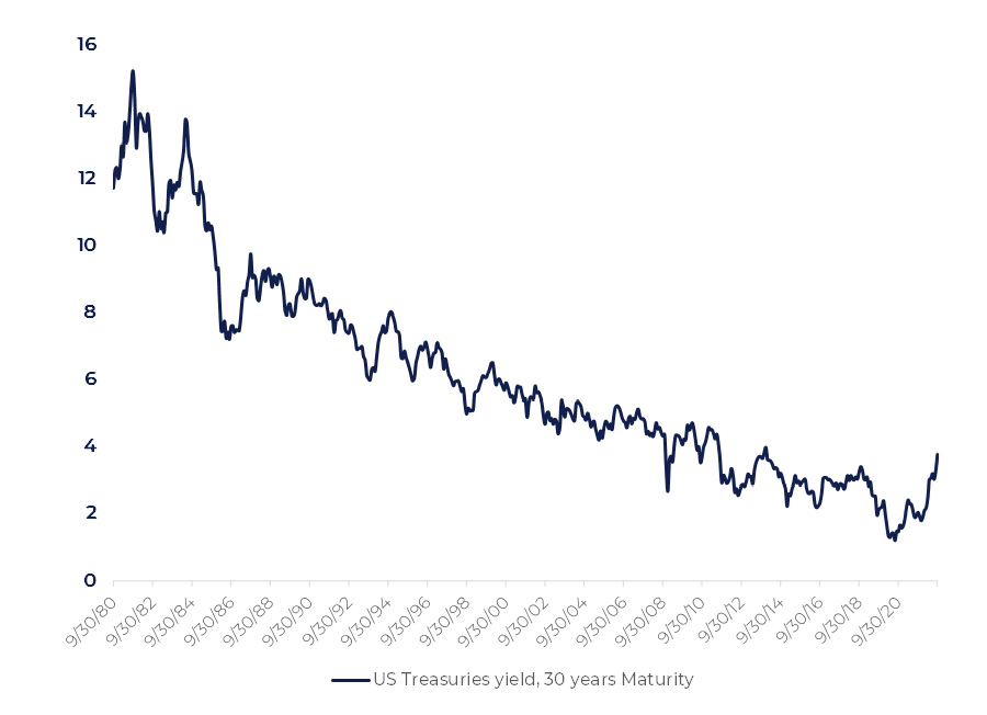
During August—September 2022 2-year US Treasuries rose almost 140bp with 30-year bonds’ yields rising as much as in Paul Volker’s era (Figure 32).
Loan rates in banks are following US Treasury bonds. As the spread between 2-year bonds (4.2%) and core PCE (4.56%) has declined to less than 50bp we have already come close to an equilibrium.
Figure 32
As we can see, the statistics is mixed, and the signals are opposite: the substantial drop of Mortgage Applications comes along with strong factory orders. With the time we are getting more positive surprises, but the equilibrium is quite shaky. All investors can do in this situation is to get their eyes focused on these figures. The less negative surprises we have the larger the equity market potential becomes.
Fundamental picture
In an ideal world reducing the excessive demand will not affect producers negatively. As an example, if an economy can only produce 1m of washing machines but there is a demand for 1.1m of washing machines, reducing the demand back to 1m will not hurt a washing machine maker.
The real life is more complicated. The money excess is distributed unevenly across the economy. There are large tech companies such as Microsoft or Apple whose earnings have soared over the past 3 years. Such companies have positive cash positions, so the monetary tightening does not affect them directly. On the other hand, there are companies such as Stanley Black and Decker whose profits were dented by surged commodity prices and revenues hit by possible slowdown in construction. The net debt level of such companies generally stands at 2—5 of EBITDA. The rate hike of 3% will reduce earning margins of such companies by another 2—3%.
Someone will get extra profits, someone will pay. The danger is that the monetary tightening will hit vulnerable companies more than they can tolerate, so that it will cause a chain reaction in the economy.
To understand these risks better it makes sense to look at 2001 in more detail.
2001 Recession
Figure 1 at the beginning of this review reveals a technical similarity of 2001 and 2022 patterns for tech stocks. IT stocks started falling in 2000, but their profits were mostly hit in 2001 (Figure 33):
Figure 33
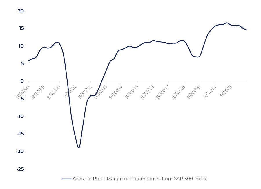
Fundamental figures followed the market partly because IT companies were trapped by closed financial markets. Many of them were cashflow-negative. They quickly turned into a cost-saving mode.
The broader picture of the 2001 goes beyond dot-com companies. Problems emerged as early as in 1997 in the Manufacturing sector.
The 1990-s was a period of strong economic growth. By 2000 capital expenditures of manufacturers soared (Figure 30). Being confident about their future, the industrial companies were rapidly increasing capital investments. The capacity utilization was weakening, however: newly installed capacities were not fully loaded.
Figure 34
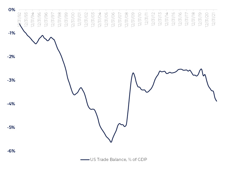
Figure 34 highlights one reason for that: US started importing goods from abroad. The drop in the US trade balance in early 2000s was mainly caused by the trade activity with China. US started using this country as a giant manufacturing plant. The US-based capacities could not compete with much more marginal Chinese production.
This led to a manufacturing’s downturn. It started in late summer of 2000 and deepened in 2001, as businesses sharply reduced spending on machinery, computers, and other capital goods. Falling orders led factories to cut more than 1 million jobs from their payrolls. This retrenchment led to job losses in wholesale trade and transportation, and to a massive cutback in factories’ use of temporary help services .
[16] U.S. labor market in 2001: economy enters a recession
The total number of employed decreased by 1.3m in Q4 2001 compared to Q4 2000. 530k of them were 16 to 19 years old. The Lowest and Middle earnings groups were hit most by the recession.
The dollar rose in 2001 to a 15-year high. The Fed reduced the key rate from 6.5% in 2000 to 1.0% in 2003. Low mortgage rates boosted the housing market and softened the slowdown in construction and real estate. This segment happened to be one of the drivers of a subsequent recovery.
Common features and differences between 2001 and 2022 patterns
As it was mentioned, the technical patterns of 2001 and 2002 look astonishingly similar. The fundamental picture is quite different, though.
First off, the Federal Reserve conducted monetary easing in 2001 while 2022 is a year of tough monetary tightening. As it was mentioned in the previous section, low-rate environment helped the construction sector recover in 2001. Another difference, though, is that in 2022 there is much excessive money in the economy already.
Second, the manufacturing sector was overcapitalized in 2000. This led to imbalances which blew up the situation. Now the manufacturing sector is undercapitalized and working at its full capacity. It is very hard to wait massive layoffs from the manufacturers in this situation.
A very interesting picture can be observed in a car making sector. Average monthly US car sales (13m) is 20% lower than that before the pandemic (17m). Individuals cannot afford buying expensive durables because they are forced to pay large bills for the fuel, electricity, and food. High interest rates make it even more complex. On the other hand, the supply chain issues are not fixed so far, resulting in scarcity in the car market . As a result, prices have gone up by 15% and stabilized car makers’ revenues. As a result, 2022 earnings of US car producers are expected to be at a historically record level.
If inflation goes down, the gross margin and the revenue growth will soften. At the same time, consumers will have more resources to buy durable goods.
To find a possible reason for a recession we should identify a weakness in an economy which is generally accompanied by some imbalances. Imbalances that were typical for 2001 do not present today.
[17] https://mercercapital.com/auto-dealer-valuation-insights/2022-how-is-the-auto-industry-doing/#:~:text=Most%20analysts%20predicted%20vehicle%20sales,would%20gradually%20improve%20in%202022
The weak point today is different. The Fed is trying to hurt individuals and firms by skyrocketing interest rates. The rise in unemployment is one of the major targets. As it is described above, the key figure here is a vacancy rate. To lower the vacancy rate, the Fed must hit businesses’ profits: otherwise, it is not clear why firms should stop hiring.
Figure 35 confirms this statement: almost all US recessions followed extended periods of shrinking corporate profits share in GDP. The unemployment rate was decreasing within these periods. The start of recession generally comes in parallel with the reversal of unemployment. Then, during the recession period, the unemployment is growing with corporate profits bottoming out. Recessions end when the unemployment reaches its highest point.
Figure 35
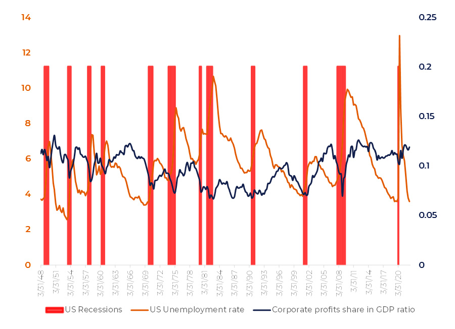
Generally, it takes more than a year for recessions to start after the turnover point of corporate profits. 2022 is an outstanding year when stocks have dropped and priced the recession in with corporate profits being on top. It is also unlikely that we will see the uptrend in unemployment in the nearest future.
It is noteworthy that falling inflation generally cause upward pressure on corporate profits . That was the case in 1971, 1974, 1984. This means that if the inflation trend proves negative the corporate profits should be at least stable. We should keep in mind that even if corporate profits share falls 20% the nominal GDP will rise the same 20-25% due to inflation. Therefore, nominal corporate profits have a limited downside.
In some sectors hiring activity has already fallen: first, it concerns technological companies for which capital markets are closed now. Messages on staff expansion limitations were sent by Meta, Shopify, and other companies of this sector. For many of them the expectations of a recession are the major argument. The Fed’s hawkish stance is an anti-inflation factor.
There are opposite examples: global airlines are still understaffed by ~10%. Such companies will support the labor market in future.
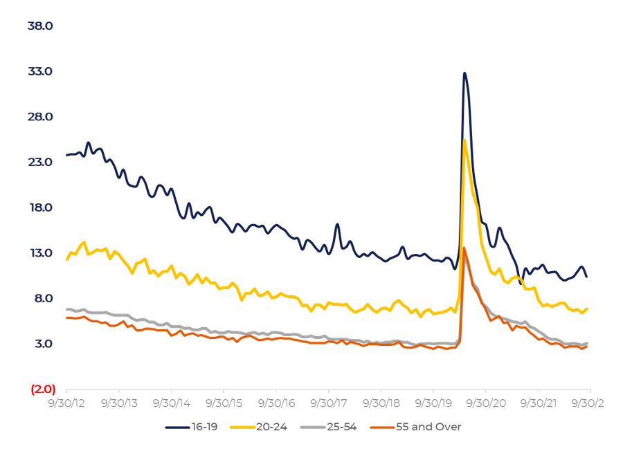
Figure 36. US Unemployment structure by age
[18] Statistically, corporate costs are more volatile than products prices. When inflation is going up the cost side dominates in balance sheets, this results in margins contraction. Visa versa, falling inflation brings about margin expansion.
Figure 36 reveals that the most imbalanced unemployment pattern is within the 16-19 age population group, indicating that the temporary and help job segments are most overheated.
Figure 37 shows the breakdown of US unemployment by education, once again pointing the hot labor market in the less educated population segment. Interestingly, the respective curve reveals some signs of normalization.
As it was mentioned above, temporary and help staff were hit the hardest by 2001 recession. Rise of unemployment in these segments will bring labor closer to its balanced state.
Figure 37. US Unemployment structure by education
There is a danger that rising unemployment will result in decline of demand more than necessary. This will hit businesses, launching a recession feedback loop. However, the monetary excess serves as a damper in current situation, softening the negative impact of rising unemployment.
Slack labor market now is sooner a result of recession expectations, not the lack of demand. High interest rates have limited impact. The 2-years US Government bonds are roughly 200bp higher than in 2018—2019. US corporate debt is roughly a half of GDP. So, US corporates pay 1% of GDP more for their debt than before COVID. As Figure 35 shows, total corporate profits are 12% of GDP. That gives a direct impact from the interest rate side of 8% decrease of earnings for US corporates.
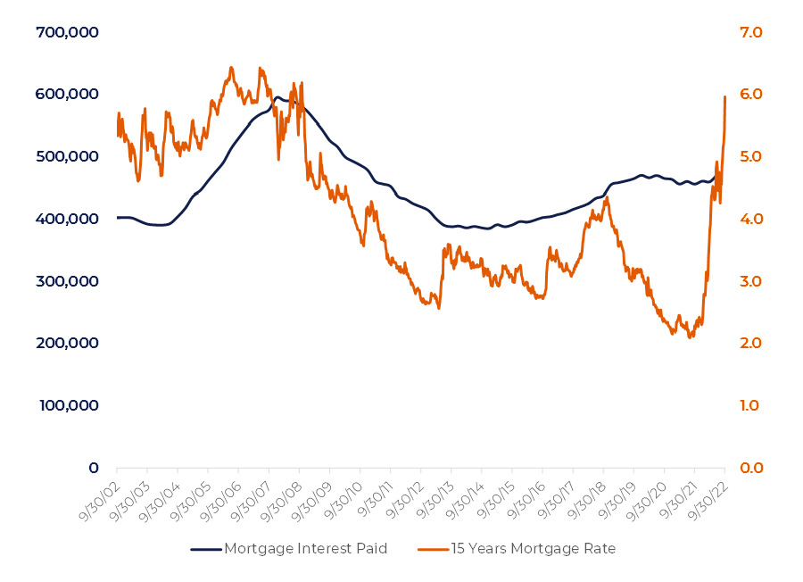
Right after the rate hike the actual impact will be much less because it will take time for old loans and bonds to rollover. Figure 38 demonstrates this on a mortgage market example.
Figure 38
US corporate debt counts for 50% of GDP, mortgages – another 50%, consumer credit – 18% of GDP. Compared to the pre-pandemic level the interest rates are about 2% higher. Assuming that the loans will be prolonged within the next 4-years period, we can roughly estimate the direct impact of a rate hike on households and businesses at 0.5% which, being applied to the total debt (120% of GDP), constitutes 0.6% of GDP.
Given that the monetary excess stands at about 17% of GDP, the direct impact of the Fed’s rate hike is very limited. It will cause the slowdown of US economy but will not affect the total amount of money.
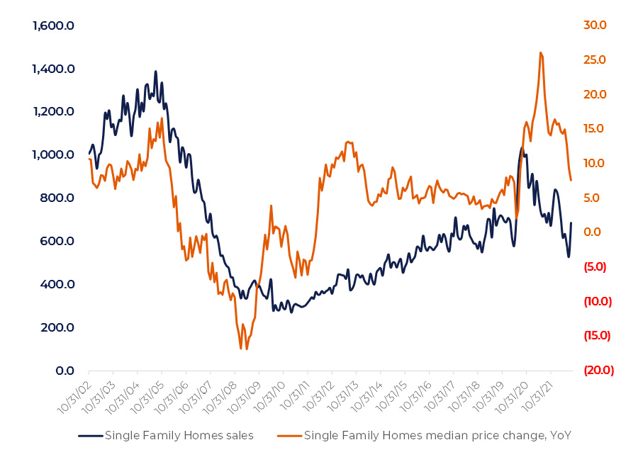
Therefore, the major effect from raising rates is discouraging companies and individuals from taking new loans but not absorbing money through interest payments. The house market has been cooling down since mid-2021: much before the Fed started acting (Figure 39). Raising rates, the Federal Reserve wants to secure the way things are developing on their own.
Figure 39. Single Family Homes sales and prices
Other factors
International trade
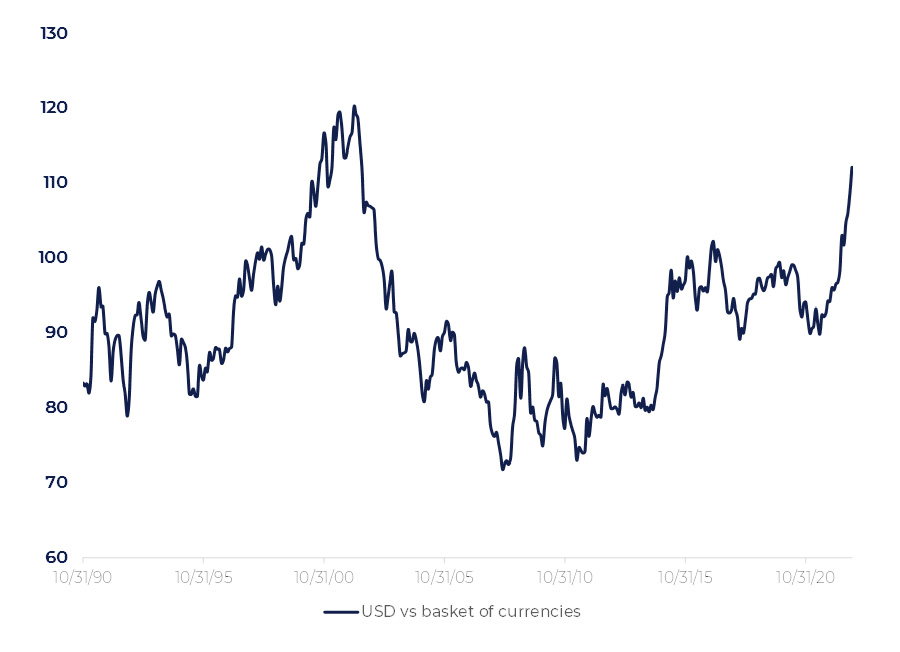
Like in 2001, dollar is very strong in 2022 (Figure 40). This directs consumer demand to the benefit of imported goods. Due to this the US Trade balance has slipped from (-$580bn pa) before pandemic to almost a minus trillion dollars in 2022. It smoothed the lack of supply and, hence, inflationary pressure.
On the other hand, expensive dollar makes US goods uncompetitive. US consumers switched to foreign goods sending US GDP growth below zero.
US companies with dollar-nominated costs selling products or services globally have to reduce their profit expectations. Almost all Tech companies are affected by strong dollar in this way. This, in turn, helps the Fed shape negative expectations.
Figure 40
It should be kept in mind that a negative trade balance means that dollars return to US in other form. It might be money on accounts, financial instruments, or direct investments from abroad. We can get the answer looking at “US Treasury bonds total foreign holdings”: it has risen from $7bn as of the beginning of 2021 to $7.5bn in August 2022. This corresponds to the $0.5bn decrease in the US trade balance.
This is an amazing chain where printed money is sent abroad and return afterwards as foreign investments in US government bonds.
Commodities
CommoditiesCommodities first rose in 2021 on supply chain constraints. The Baltic Dry index which reflects global transportation environment reached its highest level in October 2021 (Figure 41). The transportation constraints eased then but a new impetus for commodities was caused by the Russian-Ukrainian war.
Figure 41
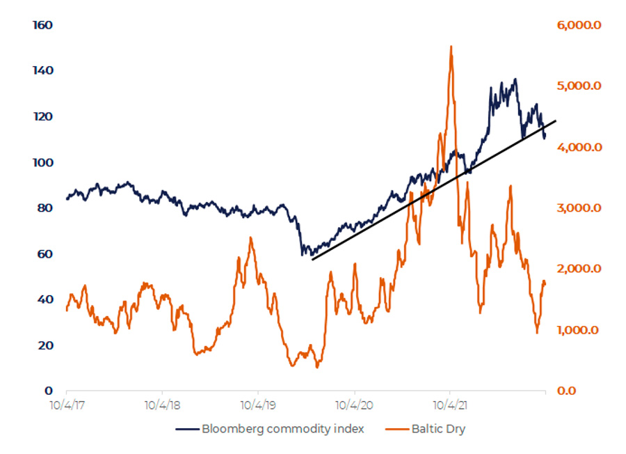
It sent commodity prices even higher. Since Summer 2022 the commodity market started revealing weakness. Bloomberg commodity index broke its technical support (Figure 41). Oil dropped below $90/bl despite OPEC’s decision to cut production in August 2022. European gas stayed steady even after the breakdown of both North Streams.
So far these are only first signs of depression in commodity market. Ongoing war means the upside risk is still high.
Commodities are often referred to as a key reason for global inflation. It is not completely the fact. Inflation takes place in countries which have conducted huge monetary emissions. China is an example of a country that have not done that, at least in the US scale. So, current CPI level in China is 2.5%.
More globally commodities are in a long-lasted downtrend starting in 2008. This commodity cycle is closely related to the business environment in Emerging Market countries. Economy growth there is much below pre-2008 levels. Now we are living in a period of recurring devaluations in Emerging Markets. Since most Emerging Market countries are exporting commodities their currencies’ weakness pressure costs of mining down. On the other hand, the breakeven cost of shale oil in US is at $$40-50 range. Considering the green shift of energy consumption in US, it is very difficult to find reasons for commodities to grow soon.
Of course, there is at least one positive driver for commodities: printed money. As the total accumulated inflation since 2020 is expected to be around 25—30%, the neutral level for commodities should be ~30% higher than before 2020. With this taken into consideration, we are near balanced level in commodity markets. Recession expectations, however, affect commodities negatively.
Various factors
The lessons of 2001 and 2008 demonstrates that S&P 500 index can lose ~45% of its value in case of a heavy recession. With the current drawdown of ~25% another 20% is remaining. The principle “never play against Fed” tells us that the further market decline is quite probable. Fed Chair Powell points to high chances of hard landing. This pushes a lot of investors to sell stocks: the situation will only become worse.
Figure 42
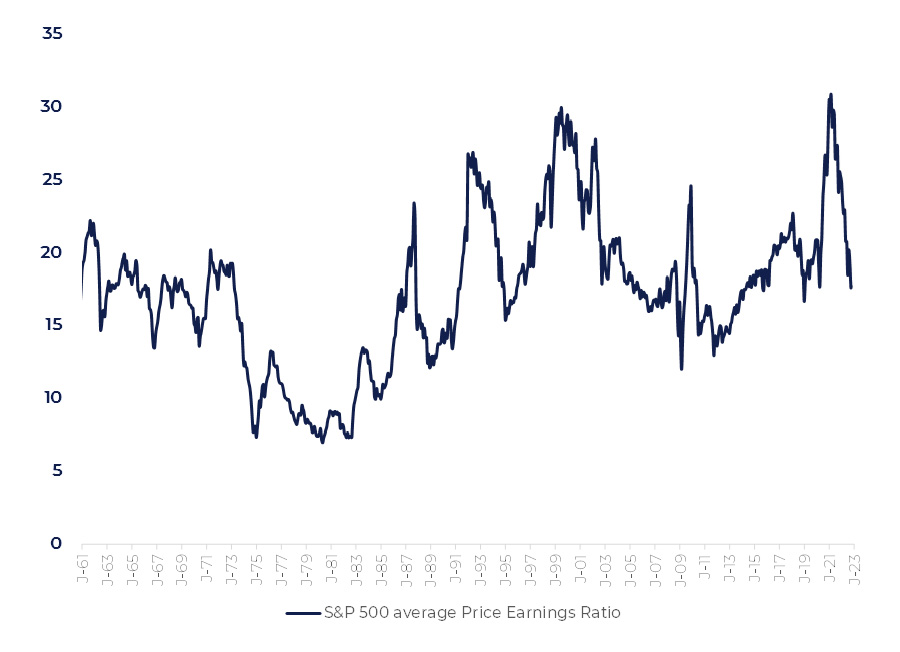
Average Price/Earnings ratio of US equity market is near 17 which witnesses the undervalued or, at least, properly valued market.
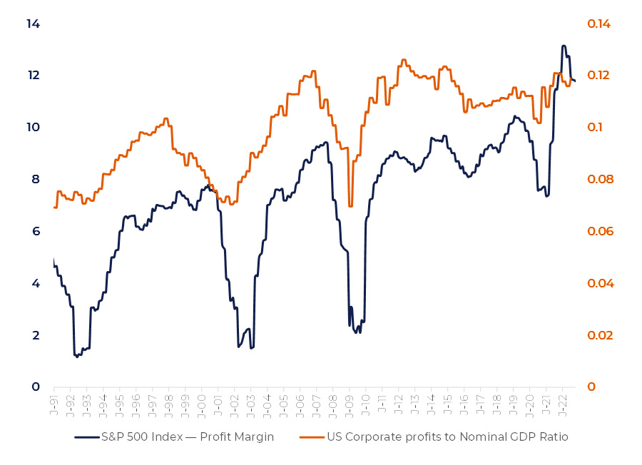
Net income margin of US stocks is at a historically record high level of 12. It is likely that strong margins are supported by inflationary demand and will contract by 10—20%. On the other hand, inflation will drive revenues up which will offset the margins’ contraction (Figure 43). US Corporate Profits will remain stable, but its share in the GDP structure will probably decline by the same 10-20% . It is bad news for stocks, although it is much less than we had in 2001 and 2008. For further 15—20% stocks downside we would rather expect more substantial drop of corporate profits to ~8% of the GDP structure.
Figure 43
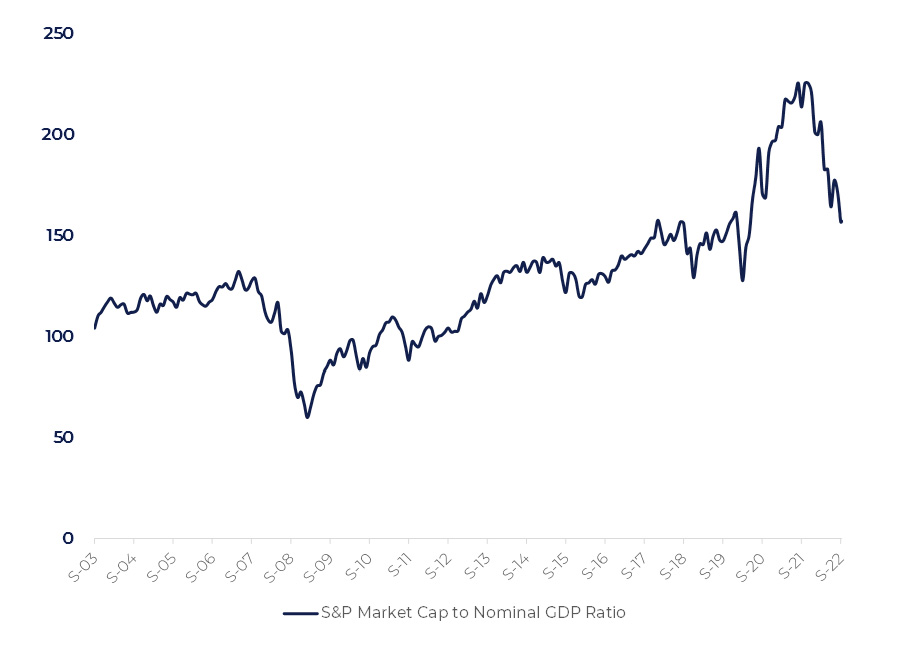
The S&P 500 market capitalization looks a bit overvalued compared to GDP (Figure 44) . After the money excess will be absorbed by the economy the ratio will go down to ~135 which is more like the bottom range.
As we can see, US equities have entered into a valuation zone which is sooner close to a balance rather than overvalued.
[19] Assuming constant corporate profits and Nominal GDP growing in line with inflation [20] This ratio is also known as “Buffet Ratio”.
Figure 44
Summary
It looks like there are many factors favoring prices cooling down on their own:
- The monetary excess will be absorbed naturally within the next two years.
- Commodity market reveals signs of weakness. Even if commodities remain at current levels the effect if high base will come into force in 2023.
- Inflation cyclicity also points to possible downturn.
- International trade smoothens inflation.
- Labor market depends on the monetary excess. The excess of job vacancies is going to decrease.
- Recession expectations are also anti-inflationary by nature.
- Fundamental valuations are closer to equilibrium even with the potential earnings downside taken into account.
However, there are risks that something will go wrong. The danger might come from soaring debt-driven consumer consumption, Russian-Ukraine war, or other black swans. To secure that inflation is under control, the Fed is going to conduct tight monetary policy in months to come.The Fed is focused on “core inflation” which is slow moving and will be rising at least until the beginning of 2023. This will maintain pressure in the markets.
The main question is whether the Fed can solve the inflation problem without a hard landing which would mean a fall of corporate profits followed by a serious growth of unemployment. The closest technical pattern is a recession of 2001. We showed that currently there are no imbalances that led to that recession. The money excess being a major inflation driver, is a support for economy at the same time. The unemployment will grow in labor market segments which have benefited most from the monetary excess. The serious growth in the unemployment rate is not likely to happen without recession.
The recession (or hard landing) is possible in case the Fed’s rate hike brings too many businesses on a brink of bankruptcy. The industrials heavy loaded with debt are most vulnerable to this. However, so far, their state seems solid.
The dangerous period will last until Q1 2023. If no substantial bankruptcies happen until then and if the core inflation will prove under the Fed’s control the markets can switch into a growing mode. The upside potential is huge.
In case of a hard landing S&P 500 has still a downside of 20%. However, the upside risk is large now as current valuations almost completely ignore chances for a soft landing.